Probability Density Function, f(x), completely describes the probability that a Random Variable, X, assumes a value in a given range of possible values.
Mathematically, the probability that random variable X, assumes a value that lies in the interval [a,b].
The above equation represents the area under the curve f(x) from a to b. The limits of the above integral depend upon the domain of the f(x). However, the total area under the curve must not be greater 1 whatever the limits are. That is
Another jargon often used with Probability Density Function is Cumulative Distribution Function (cdf). As the name implies it is the cumulative probability that a random variable X takes on a value equal or less than some specific value. For given value a, F(a) is the Cumulative Distribution Function that shows the probability that the random variable X assumes a value equal to or less than a. Mathematically shown as below
P(X < a) = F(a) ………….(3)
Cumulative Distribution Function is based on probability, it has following properties:
0 <= F(a) <=1
F(a1) <= F(a2) if a1 < a2
F(-∞) = 0
F(+∞) = 1
The relationship between Cumulative Distribution Function (cdf) and Probability Density Function (pdf) is shown below
That means the value of the F(a) is equal to the area under probability density function curve upto a.
From the above relationship, conversely, we have
Above two equations give us the relationship between cdf and pdf.
Following links provide a very simple understanding of pdf and cdf:
Now for Probability Density Function of a sine wave. Let’s say we have
X = sin(Y) ………………… (6)
A sine wave has been shown in figure below:

For equation (6), we already know that Y is uniformly distributed over [- pi/2 , pi/2] so X takes on a value in the range [-1, 1]. In this case, X is our random variable for which probability density function is given by eq (1). We aim to find the function f(x) for the sine wave given in eq (6).
Generally the inverse of a function provides the distribution of the values of that function which can be converted into Cumulative Distribution Function (cdf) after a little manipulation. These manipulations are done so that it fits with the definition of cdf.
We have random variable X which can assume a value in the interval [-1, 1]. Therefore
P(X < a) = P (sin(Y) < a) = P(Y < arcsin(a)) where -1<=a<=1
Hence
Notice the modifications of dividing factor of and additive factor of ½ which have been done to make it compliant with the definition of Cumulative Distribution Function and its properties shown above.
Cumulative Distribution Function of a sine wave is shown below:
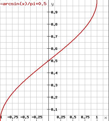
The possible values that a sine function can assume are shown along X-axis while probability is shown along Y-axis. The maximum probability can be 1.
Now making use of equation (5) above, we can calculate the Probability Density Function (pdf) of sine function (sine wave) by taking the derivative of equation (7). Hence pdf of sine wave is given below

This is quite intuitive that as the slope of a function increases at a value, the chances of occurring that value are higher. (Think of a straight line parallel to Y-axis which has infinite slope and has only one value occurring all the times along X-axis). The probability density function (pdf) of a sine wave, f(x), is shown below:

The pdf shows that probability is high near the extreme values of -1 and 1 as most of the possible values occur towards the extreme values. For example, sine function reaches at 0.5 (half of its max amplitude) just at pi/6 (i.e. 30 degrees).
All the above plots have been created from rechneronline.